We will be exploring a simple yet powerful trick to extract the last word from any cell in Microsoft Excel. The beauty of this method is that it only requires a single formula; no macros or add-ons are necessary. Let’s dive right in!
Get last word: understanding the formula
The formula we are using is:
=TRIM(RIGHT(SUBSTITUTE(A2," ",REPT(" ",50)),50))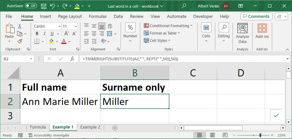
Which returns “Miller”. This formula is a combination of three primary functions: SUBSTITUTE, RIGHT, and TRIM. Here’s a quick rundown of each component:
- SUBSTITUTE Function: This is the first part of our formula, where we replace every space in the cell with 50 spaces, using the
SUBSTITUTE(A2," ",REPT(" ",50))segment of the formula. In this segment, A2 is the reference for the cell containing the text from which we want to extract the last word. - RIGHT Function: Following the SUBSTITUTE function, we have the RIGHT function, which incorporates the functionalities of the SUBSTITUTE function and extends up to the second number 50, denoted as
,50in the formula. This part of the formula extracts the last 50 characters from the cell, encompassing the last word along with numerous spaces. - TRIM Function: Finally, we employ the TRIM function to eliminate all the extra spaces, leaving us with only the last word. This is represented by the
TRIM(...)portion of the formula.
You might wonder why the number 50 is used in this formula. The reason is quite straightforward: there are no words in the English language that exceed 50 characters, making this a safe number to use to ensure we capture the last word fully.
Example use cases
Now that we have a grasp of the formula’s components, let’s see it in action with a couple of examples in the video below:
Conclusion
As we have seen, this formula is not only powerful but also dynamic, adjusting to extract the last word even when additional words are added to the cell. I hope you found this tutorial helpful!